
My previous paper pointed out that ancestry is important for understanding the genetic diversity of cancer cell lines and their implications for therapeutic responses. This tutorial outlines the computational pipeline that I derived to reliably classify cancer cell lines into ancestries based on genotype data. The pipeline consists of three key stages: data processing, quality control, genotype imputation, and ancestry inference, each explained in detail to guide its implementation.
Disclaimer: The paper was written in 2019 as part of a project whose main goal was to evaluate the impact of ancestry to drug response in cancer cell lines. Today there might be more advanced ancestry inference methods, applied not only to cancer cell lines. It would be interesting to see the performance of our method in comparison to the more recent methods.
Preparation
I first created a few folders in the working directory as following, and put the raw data into the data folder:
|--- working dir
   |--- data # Raw data
   |--- transformed # Plink text files (PED, MAP, FAM)
   |--- plink # Plink binary files (BED & BIM)
   |--- qc # QCed data
   |--- input # Input for ancestry reference
   |--- reference dir # All reference files
        |--- legend/1000GP_Phase3_combined.legend
        |--- vcf
        |--- m3vcf
        |--- bcf
        |--- map/genetic_map_hg19_withX.txt
I also set up a few things before the main process. First I downloaded 1000 Genome Project’s reference VCF files for all populations and put to reference dir/vcf/, legend file and put to ref dir/legend/, genetic map file and put to ref dir/map.
I also installed the following software in advance: R, R packages ggplot2, dplyr, biomaRt and stringr, Perl, Ensembl API, Eagle2, minimac3, minimac4. You can check out this Dockerfile that I used to install these softwares.
Finally, I put the following utility R scripts in the working directory which will assist the subsequent analyses:
check_position.R:
    #!/usr/bin/env Rscript

    args <- commandArgs(trailingOnly=TRUE)

    sample <- read.table(args[1], header = F, sep = "\t")
    ref <- read.table(args[2], header = F)
    index <- match(sample$V4, ref$V1)
    index_unmatched <- is.na(index)
    unmatched_position <- sample[index_unmatched,]
    write.table(unmatched_position, file = "qc/unmatched_position.txt", row.names = F, col.names = F, quote = F)
check_refalt.R:
    #!/usr/bin/env Rscript

    args <- commandArgs(trailingOnly=TRUE)

    sample <- read.table(args[1], header = F, sep = "\t", stringsAsFactors = F)
    ref <- read.table(args[2], header = F, stringsAsFactors = F)
    ref <- ref[match(sample$V4, ref$V1),]

    for (i in 1:nrow(sample)){
        sam_ref <- sample$V6[i]
        sam_alt <- sample$V5[i]
        ref_ref <- ref$V2[i]
        ref_alt <- ref$V3[i]

        if (sam_ref == ref_ref && sam_alt == ref_alt){
            next
        } else if ( sam_ref == ref_alt && sam_alt == ref_ref){
            next
        } else {
            cat(paste(sample[i,2]), file="./qc/unmatched_alleles.txt", append=TRUE, sep = "\n")
        }
    }
Data preprocessing
The first step in the pipeline involves data processing to prepare genotype data for subsequent analysis. In our case, the input data were in CSV format of the Affymetrix SNP6.0 arrays containing 1007 cancer cell lines and 884,148 SNPs ranging from chromosome 1 to chromosome 22, which are deposited in the European Genome-Phenome Archive (EGAS00001000978). Particularly, there was one CSV file per cell line, of which rows were SNPs and columns were he SNPs’ features. Below is an example of an input CSV (not a real cell line and only 5 rows are shown):
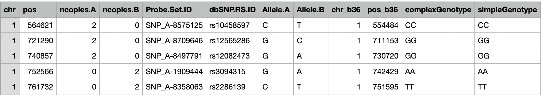
Example CSV file for genotypes of cancer cell lines
The data was first transformed into PLINK file formats (PED, MAP, BED, BIM, and FAM), which are suitble for subsequent genomic analyses. During preprocessing, CSV text files were manipulated through multiple steps to output appropriate PLINK formats. Run the following code for data processing:
    WDIR=[working directory]
    DDIR=[data directory]
    REFDIR=[reference directory]
    LEGFILE=${REFDIR}/legend/1000GP_Phase3_combined.legend
    VCFFILE=${REFDIR}/vcf
    MAPFILE=${REFDIR}/map/genetic_map_hg19_withX.txt

    ###Transform genotyping files into .ped and .map files and arrange in chromosomes
    for chr in {1..21}
    do
        for file in  ${filename[@]}
        do
            #Filter for chromosome and add whitespace within geneotypes
            awk -F "\"*,\"*" -v chr=$chr '$1==chr{print $12}' $DDIR/$file | sed 's/./& /g' > tmp.txt

            #Add '0' to missing geneotypes
            awk '!$1 { $1="0 0 " }1 ' tmp.txt > tmp_filled.txt

            #Flip column -> row
            paste -s -d "" tmp_filled.txt > tmp_flipped.txt
            echo "$file" > cell_name_tmp.txt

            #Remove unneccesary part in cell name
            perl -pi -e 's/_complexGenotypes.csv//g' cell_name_tmp.txt
            paste -d " " cell_name_tmp.txt tmp_flipped.txt >> chr"$chr"_tmp.txt
        done

        awk '{print $1}' chr"$chr"_tmp.txt > cell_name.txt
        cut -f1 -d " " --complement chr"$chr"_tmp.txt > chr"$chr"_tmp_trimmed.txt

        while IFS= read -r line; do
            #Create essential fields for the .ped file
            echo "1 $line 0 0 0 0" >> chr"$chr"_prefix.txt
        done < cell_name.txt

        #Make .ped file
        paste -d " " chr"$chr"_prefix.txt chr"$chr"_tmp_trimmed.txt > ./transformed/chr"$chr".ped

        #Make .map file
        awk -F "\"*,\"*" -v chr=$chr '$1==chr{print $1, $6, $2}' $DDIR/8-MG-BA_complexGenotypes.csv > ./transformed/chr"$chr".map

        #Remove rows (cell lines) with fewer columns than expected (unknown technical error)
        cp ./transformed/chr"$chr".ped ./transformed/"$chr".ped
        max=$(awk '{print NF}' ./transformed/"$chr".ped | sort -n | tail -n 1 )
        awk -v MAX=$max 'NF==MAX{print}' ./transformed/"$chr".ped > ./transformed/chr"$chr".ped
        rm ./transformed/"$chr".ped

        #Make plink binary files
        ./plink --file ./transformed/chr"$chr" --make-bed --out ./plink/chr"$chr"
        ./plink --freq --bfile ./transformed/chr"$chr" --out ./plink/chr"$chr"
    done
Quality control
The transformed data was then checked for its quality before imputation. During quality control, SNPs with more than 10% missing data or minor allele frequencies below 0.05 were excluded. The positions of retained SNPs were compared against a legend file of the same reference build from the 1000 Genomes Project, and any mismatched SNPs were removed. Additional steps were taken to identify and exclude SNPs with inconsistencies such as reference strand swapping, alternate allele mismatches, or strand flipping, ensuring only high-confidence data remained for downstream analyses. Run the following code to execute quality control:
    for chr in {1..21}
    do
        # Checking genotyping rate, MAF and HWE integrity
        plink --bfile ./plinkd/chr$chr --silent --missing --out ./qc/chr$chr
        sed 1d ./qc/chr${chr}.lmiss | awk '{if ($5 > 0.1) print $2,$5}' > ./qc/chr${chr}_missing_snps.txt
        if [[ -s ./qc/chr${chr}_missing_snps.txt ]]
        then
            echo "These SNPs have larger than 10% missing rate (see complete list in ./qc/chr${chr}_missing_snps.txt):"
            cat ./qc/chr${chr}_missing_snps.txt | head
            echo '...' | sed G
        else
            echo "All SNPs have higher than 90% typing rate" | sed G
        fi
        plink --bfile ./plinkd/chr${chr} \
        --silent \
        --geno 0.1 --recode --out ./qc/chr${chr}_freqfiltered

        #SNPs with unmatched positions
        #Checking positions compared to reference legend file
        cat ${LEGFILE} | awk -v CHR=${chr} '{if ($2==CHR && $6=="Biallelic_SNP") print}' > ./qc/ref_chr${chr}.txt
        awk '{print $3}' ./qc/ref_chr${chr}.txt > ./qc/ref_chr${chr}_coord.txt
        echo "Reference legend written to ./qc/ref_chr${chr}.txt and ./qc/ref_chr${chr}_coord.txt" | sed G
        Rscript --vanilla check_position.R ./qc/chr${chr}_freqfiltered.map ./qc/ref_chr${chr}_coord.txt
        awk '{print $2}' ./qc/unmatched_position.txt > ./qc/chr${chr}_unmatched_position.txt
        if [[ -s ./qc/chr${chr}_unmatched_position.txt ]]
        then
            echo "SNPs having unmatched positions (see complete list at ./qc/chr${chr}_unmatched_position.txt):"
            cat ./qc/chr${chr}_unmatched_position.txt | head
            echo '...' | sed G
            echo Removing these SNPs... | sed G
            plink --file ./qc/chr${chr}_freqfiltered --silent --exclude ./qc/chr${chr}_unmatched_position.txt --recode --out ./qc/chr${chr}_posfiltered
        else
            echo All SNPs have correct positions | sed G
            plink --file ./qc/chr${chr}_freqfiltered --silent --recode --out ./qc/chr${chr}_posfiltered
        fi

        #Check REF/ALT and flip strands
        awk '{print $3,$4,$5}' ./qc/ref_chr${chr}.txt > ./qc/ref_chr${chr}_alleles.txt
        echo "Legend alleles are written to ./qc/ref_chr${chr}_alleles.txt" | sed G

        ##Checking unmatching and flipping...
        rm -f ./qc/swapped_alleles.txt ./qc/unmatched_alleles.txt
        plink --file ./qc/chr${chr}_posfiltered --silent --make-bed --out ./qc/chr${chr}_posfiltered
        Rscript --vanilla check_refalt.R ./qc/chr${chr}_posfiltered.bim ./qc/ref_chr${chr}_alleles.txt
        cp ./qc/unmatched_alleles.txt ./qc/chr${chr}_unmatched_alleles.txt
        if [[ -s ./qc/chr${chr}_unmatched_alleles.txt ]]
        then
            echo "These SNPs have invalid REF/ALT alleles (see complete list at ./qc/chr${chr}_unmatched_alleles.txt):"
            cat ./qc/chr${chr}_unmatched_alleles.txt | head
            echo '...' | sed G
            echo Removing them... | sed G
            plink --bfile ./qc/chr${chr}_posfiltered --silent --exclude ./qc/chr${chr}_unmatched_alleles.txt --make-bed --out ./qc/chr${chr}_QCed
        else
            echo No invalid alleles found | sed G
            plink --bfile ./qc/chr${chr}_posfiltered --silent --make-bed --out ./qc/chr${chr}_QCed
        fi
        echo "Finish QC check for chromosome ${chr}. Final QCed files at ./qc/chr${chr}_QCed" | sed G | sed G
    done
Imputation
After quality control, we needed to impute the missing genotypes that were not included in the Affymetrix detection. This is an important step since the SNPs of our interest (involved in the ancestry inference) were not detected in the original dataset. To this end, the binary file sets were converted into VCF files using PLINK. A reference genome in the form of phased VCF files was obtained from the 1000 Genomes Project at the beginning and subsequently converted to BCF format using BCFtools and to M3VCF format using Minimac3. The input VCF files were phased using Eagle2, utilizing the BCF reference files and the genetic map from the 1000 Genomes Project. Once phased, the VCF files were imputed with Minimac4 to fill in missing SNPs on each chromosome, relying on the M3VCF reference genome for accurate predictions.
    WDIR=[working directory]
    DDIR=[data directory]
    REFDIR=[reference directory]
    LEGFILE=${REFDIR}/legend/1000GP_Phase3_combined.legend
    VCFFILE=${REFDIR}/vcf
    M3VCFFILE=${REFDIR}/m3vcf
    BCFFILE=${REFDIR}/bcf
    MAPFILE=${REFDIR}/map/genetic_map_hg19_withX.txt

    echo Creating BCF reference and target files for phasing... | sed G
    for chr in {1..21}
    do
        echo Creating indexed BCF files for chromosome ${chr}...
        bcftools view ${VCFFILE}/ALL.chr${chr}.phase3_shapeit2_mvncall_integrated_v5a.20130502.genotypes.vcf.gz -O b -o ${BCFFILE}/ref_chr${chr}.bcf
        bcftools index ${BCFFILE}/ref_chr${chr}.bcf
        plink --silent --bfile ./qc/chr${chr}_QCed --recode vcf-iid bgz --out ./input/chr${chr}
        bcftools view ./input/chr${chr}.vcf.gz -O b -o ./input/chr${chr}.bcf
        bcftools index ./input/chr${chr}.bcf
    done

    echo Phasing... | sed G
    for chr in {1..21}
    do
        echo Phasing chromosome ${chr}...
        eagle --vcfRef ${BCFFILE}/ref_chr${chr}.bcf \
                --vcfTarget ./input/chr${chr}.bcf  \
                --geneticMapFile ${MAPFILE} \
                --outPrefix ./phased/chr${chr}.phased \
                --allowRefAltSwap \
                --numThreads 5 \
                --vcfOutFormat z
    done

    echo Imputing...
    for chr in {1..21}
    do
        echo Imputing chromosome ${chr}...
        minimac4 --refHaps ${M3VCFFILE}/${chr}.1000g.Phase3.v5.With.Parameter.Estimates.m3vcf.gz \
                --haps ./phased/chr${chr}.phased.vcf.gz \
                --prefix ./imputed/chr${chr}.imputed \
                --cpus 5  \
                --noPhoneHome \
                --format GT,DS,GP \
                --allTypedSites --minRatio 0.00001
    done
After the imputation, post processing needed to be done to ensure the quality of the imputed SNPs and extract the geneotypes of the SNPs of interest. For inferring ancestry, I leveraged the set of 100 SNPs that were shown to be associated with ancestry (genetic markers) by Sampson et al.. The raw genotype data from GDSC only included 26 from the 100 SNPs, so I did the imputation as shown above to retrive the genotypes of the rest 74 SNPs. Following imputation, I got the complete genotype information of the 100 SNPs for each cell line. In order to extract the SNPs from the imputed data, I first need the names of the SNPs in a text file, saved in the working directory as 100snps.txt:
rs194014
rs1356733
rs4751629
rs1281340
rs11164559
...
The I used the text file to get the SNPs’ coordinates and other properties using the R package biomaRt, which retrived the information from the Ensembl database. The retrived information will be used to post process the imputed data. To this end I run the R script:
    #!/usr/bin/env Rscript

    library(ggplot2)
    library(dplyr)
    library(biomaRt)
    library(stringr)

    #Load 100 SNPs
    data_snp <- read.csv("100snps.txt", sep = "\t", header = F)

    #Get info from biomart
    snp_mart <- useMart(biomart="ENSEMBL_MART_SNP",
                    host="grch37.ensembl.org", path="/biomart/martservice",
                    dataset="hsapiens_snp")
    data_snp_mart <- getBM(attributes=c(
    "refsnp_id", "chr_name","allele", "allele_1", "minor_allele",
    "minor_allele_freq", "synonym_name", "variation_names"),
    filters="snp_filter", values=data_snp$V1,
    mart=snp_mart, uniqueRows=TRUE)

    #Get coordinates for 100 SNPs (for genotype imputation using other tools)
    data_snp_coord <- getBM(attributes=c(
    "refsnp_id", "chr_name", "chrom_start", "chrom_end"),
    filters="snp_filter", values=rsID_ethc,
    mart=snp_mart, uniqueRows=TRUE)
    data_snp_coord <- data_snp_coord[-grep("H",data_snp_coord$chr_name),]
    write.table(data_snp_coord, file = "snp.txt", sep = "\t", row.names = F, quote = F)
After getting the ancestral SNP coordinates, I run the following script to process the imputed results the extract the relevant SNPs for subsequenct ancestry inference:
    WDIR=[working directory]
    DDIR=[data directory]
    REFDIR=[reference directory]
    LEGFILE=${REFDIR}/legend/1000GP_Phase3_combined.legend
    VCFFILE=${REFDIR}/vcf
    M3VCFFILE=${REFDIR}/m3vcf
    BCFFILE=${REFDIR}/bcf
    MAPFILE=${REFDIR}/map/genetic_map_hg19_withX.txt
    SNP=${WDIR}/snp.txt

    for chr in {1..21}
    do
        echo Processing imputed chromosome ${chr}

        plink --vcf ./imputed/chr${chr}.imputed.dose.vcf.gz \
            --snps-only \
            --silent \
            --recode --out ./scratch/chr${chr}_filtered
        if [[ ! -s ./scratch/chr${chr}_filtered.ped ]]; then
            echo No snp passing filtering | sed G
            continue
        fi
        perl -pi -e 's/"//g' $SNP
        awk -v CHR=${chr} '$2==CHR{print}' $SNP > ./scratch/snp_${chr}.txt
        Rscript --vanilla match_ids.R ./scratch/chr${chr}_filtered.map ./scratch/snp_${chr}.txt ${chr}

        awk '{print $5}' ./scratch/snp_${chr}_withIDs.txt > ./scratch/extracted_ids_${chr}.txt
        plink --file ./scratch/chr${chr}_filtered \
            --silent \
            --extract ./scratch/extracted_ids_${chr}.txt \
            --recode vcf-iid --out ./scratch/chr${chr}_filtered_extracted
        awk '!/#|##/ {print}' ./scratch/chr${chr}_filtered_extracted.vcf > ./scratch/chr${chr}_filtered_extracted_trimmed.vcf
        awk '/#CHROM/{print}' ./scratch/chr${chr}_filtered_extracted.vcf > ./ancestral_snp/snp_imputed_${chr}.txt
        #perl -pi -e 's/0_1_//g' ./ancestral_snp/snp_imputed_${chr}.txt
        while IFS= read -r line; do
            echo $line > ./scratch/tmp.txt
            REF=$(awk '{print $4}' ./scratch/tmp.txt)
            ALT=$(awk '{print $5}' ./scratch/tmp.txt)
            perl -pi -e 's/0\/0/'${REF}''${REF}'/g' ./scratch/tmp.txt
            perl -pi -e 's/0\/1/'${REF}''${ALT}'/g' ./scratch/tmp.txt
            perl -pi -e 's/1\/1/'${ALT}''${ALT}'/g' ./scratch/tmp.txt
            cat ./scratch/tmp.txt >> ./ancestral_snp/snp_imputed_${chr}.txt
        done < ./scratch/chr${chr}_filtered_extracted_trimmed.vcf
        perl -pi -e 's/ /\t/g' ./ancestral_snp/snp_imputed_${chr}.txt
    done
Ancestry inference
The observed and imputed ancestral SNPs were leveraged to infer ancestry of the cell lines. To this end, Bayesian inference was employed to estimate the likelihood of a cell line belonging to a specific population given its observed genotypes, the genotype frequencies of the population, and their weights in the 1000 Genomes Project.
First, the population genotype frequencies were retrieved using the Ensembl API. After installing the API, I run the following Perl script to retrieve the general frequencies for the SNPs of interest:
    #One needs to install Ensembl API before using this script
    use strict;
    use warnings;
    use Bio::EnsEMBL::Registry;

    my $registry = 'Bio::EnsEMBL::Registry';

    # Load the registry from db
    $registry->load_registry_from_db(
    -host => 'ensembldb.ensembl.org',
    -user => 'anonymous'
    );

    my $va_adaptor = $registry->get_adaptor('human','variation','variation');
    $va_adaptor->db->use_vcf(1);

    my $filename = '100snps.txt';
    open(my $fh, '<:encoding(UTF-8)', $filename)
    or die "Could not open file '$filename' $!";

    my @snps = <$fh>;
    chomp @snps;

    foreach my $snps (@snps) {
    print "$snps\n";
    }

    foreach my $snps (@snps) {
    my $va = $va_adaptor->fetch_by_name($snps); #get the Variation from the database using the name
    my $genotypes = $va->get_all_PopulationGenotypes();
    foreach my $genotype (@{$genotypes}) {
    my $pop_name = $genotype->population->name;
    my $gt_name = $genotype->genotype_string;
    my $freq = $genotype->frequency;
        open (FH, '>>', 'genotypes.txt') or die "Could not open file $!";
    print FH "$snps $pop_name $gt_name $freq\n";
    close (FH);
    }
    }

    print('Write to genotype successfully!')
After running the Perl script, I got the result stored in genotype.txt in the working directory, which is a text file of four columns for SNP names, populations, genotypes and frequency, respectively, as example below:
rs194014 AFR GG 0.142208774583964 # Frequencies of the 3 genotypes of the SNP for Africans
rs194014 AFR AG 0.453857791225416
rs194014 AFR AA 0.40393343419062
rs194014 AMR GG 0.786743515850144 # Frequencies of the 3 genotypes of the SNP for Americans
rs194014 AMR AG 0.198847262247839
rs194014 AMR AA 0.0144092219020173
...
I also needed the population sizes which I obtained from the 1000 Genomes Project and use them as the population weights in my inference pipeline. You can get it here and put it in the working directory.
For a cell line \(Y_i\) with the genotype \(G_i\) derived from ancestral SNPs that occur independently, the probability \(P(G_i)\) that \(Y_i\) belongs to a specific population 𝑘 (where 𝑘 represents one of the 25 subpopulations in the 1000 Genomes Project) is calculated as follows:
\[P(\vec{G}_i) = \frac{\prod_{j=1}^{100} \hat{P}(Y_i = k) \times {P}(Y_i = k)}{\hat{P}(G_{ij})}\]The subpopulation with the highest probability was assigned to the cell line. To implement this, I run the following script:
    #!/usr/bin/env Rscript

    library(ggplot2)
    library(dplyr)
    library(biomaRt)
    library(stringr)

    #Import imputed data
    for (chr in seq(1:21)){
    file <- paste0("./ancestral_snps/snp_imputed_",chr,".txt")
    if (file.exists(file)){
        assign(paste0("snp_",chr,"_imputed"),read.delim(file, header = T, sep = "\t", row.names = NULL))
    }
    }
    cname <- colnames(snp_1_imputed)
    for (chr in seq(1:21)){
    name <- paste0('snp_',chr,'_imputed')
    if (exists(name)) {
        obj=get(name)
        obj=obj[,cname]
        assign(name,obj)
    }
    }

    snp_imputed <- do.call(rbind, lapply( paste0("snp_",c(1:21),"_imputed") , get) )
    snp_imputed$ID <- as.character(snp_imputed$ID)
    index <- match(snp_imputed$POS,data_snp_coord$chrom_start)
    for (i in 1:length(index)){
    snp_imputed$ID[i] <- data_snp_coord$refsnp_id[index[i]]
    }

    snp_imputed <- snp_imputed[,-c(1,2,4:9)]
    rownames(snp_imputed) <- snp_imputed$ID
    data_final <- as.matrix(snp_imputed[,-1])

    #Label cell lines with estimated ethnicity probability using frequencies from 1000Gen
    size_1kg <- read.csv("sample_size_1kg.csv", header = T)
    data_1kg <- read.delim("genotypes2.txt", header = F, sep = "",
                            col.names = c("rsID", "population", "genotype", "frequency"))
    data_1kg$sup_pop <- vector(mode = "character", length = nrow(data_1kg))
    data_1kg$size <- vector(mode = "numeric", length = nrow(data_1kg))
    index <- match(data_1kg$population, size_1kg$Population)

    for (i in 1:nrow(data_1kg)){
    data_1kg$size[i]<- size_1kg$Number.of.genotypes[index[i]]
    if (data_1kg$population[i]=="ALL"){
        data_1kg$sup_pop[i] <- "ALL"
    } else if (data_1kg$population[i] %in% c("ACB","AFR","ASW","ESN","GWD","LWK","MSL","YRI")){
        data_1kg$sup_pop[i] <- "AFR"
    } else if (data_1kg$population[i] %in% c("AMR","CLM","MXL","PEL","PUR")){
        data_1kg$sup_pop[i] <- "AMR"
    } else if (data_1kg$population[i] %in% c("EAS","CDX","CHB","CHX","JPT","KHV")){
        data_1kg$sup_pop[i] <- "EAS"
    } else if (data_1kg$population[i] %in% c("EUR","CEU","FIN","GBR","IBS","TSI")){
        data_1kg$sup_pop[i] <- "EUR"
    } else if (data_1kg$population[i] %in% c("SAS","BEB","GIH","ITU","PJL","STU")){
        data_1kg$sup_pop[i] <- "SAS"
    } else {
        data_1kg$sup_pop[i] <- "NA"
    }
    }
    data_1kg <- data_1kg[-grep("NA",data_1kg$sup_pop),]
    data_1kg <- data_1kg[!data_1kg$population %in% c("ALL","AFR","AMR","EAS","EUR","SAS"),] %>%
    droplevels()

    prob <- vector(mode = "list", length = ncol(data_final))
    names(prob) <- colnames(data_final)
    prob_mat <- matrix(nrow = ncol(data_final), ncol = nlevels(data_1kg$population),
                    dimnames = list(colnames(data_final),levels(data_1kg$population)))

    for (n in 1:ncol(data_final)){
    prob[[n]] <- matrix(nrow = nrow(data_final), ncol = nlevels(data_1kg$population),
                        dimnames = list(rownames(data_final),levels(data_1kg$population)))
    for (i in 1:nrow(data_final)) {
        for (j in 1:ncol(prob[[n]])) {
        sub_data <- data_1kg[as.character(data_1kg$rsID) == rownames(data_final)[i] &
                                as.character(data_1kg$population) == colnames(prob[[n]])[j], ]
        temp_index <- match(data_final[i,n], sub_data$genotype)
        if (is.na(temp_index)){
            tmp <- strsplit(data_final[i,n],NULL)[[1]]
            tmp_rev <- rev(tmp)
            data_final[i,n] <- paste(tmp_rev,collapse = '')
            temp_index <- match(data_final[i,n], sub_data$genotype)
        }
        temp_snp_freq <- sub_data$frequency[temp_index]
        temp_pop_size <- sub_data$size[temp_index]
        prob[[n]][i,j] <- as.numeric(temp_snp_freq) * as.numeric(temp_pop_size)
        }
    }
    prob_mat[n,] <- apply(prob[[n]], 2, prod, na.rm=T)
    }

    prob_vec <- prob_vec = apply(prob_mat,1,function(x) names(which.max(x)))
    cell_ancestry <- data.frame(cell=names(prob_vec), ancestry=prob_vec)
    cell_ancestry$sup_pop <- match(cell_ancestry$ancestry,data_1kg$population)
    cell_ancestry$sup_pop <- data_1kg$sup_pop[cell_ancestry$sup_pop]
    cell_ancestry$cell <- str_replace_all(cell_ancestry$cell, c("\\."="-", "^X"=""))

    saveRDS(prob_mat, file = "prob_mat.rds")
    write.table(cell_ancestry, file = "cell_ancestry.csv", row.names = F, quote = F, sep = ",")
The inferred ancestry for all cell lines in our study looks like this:
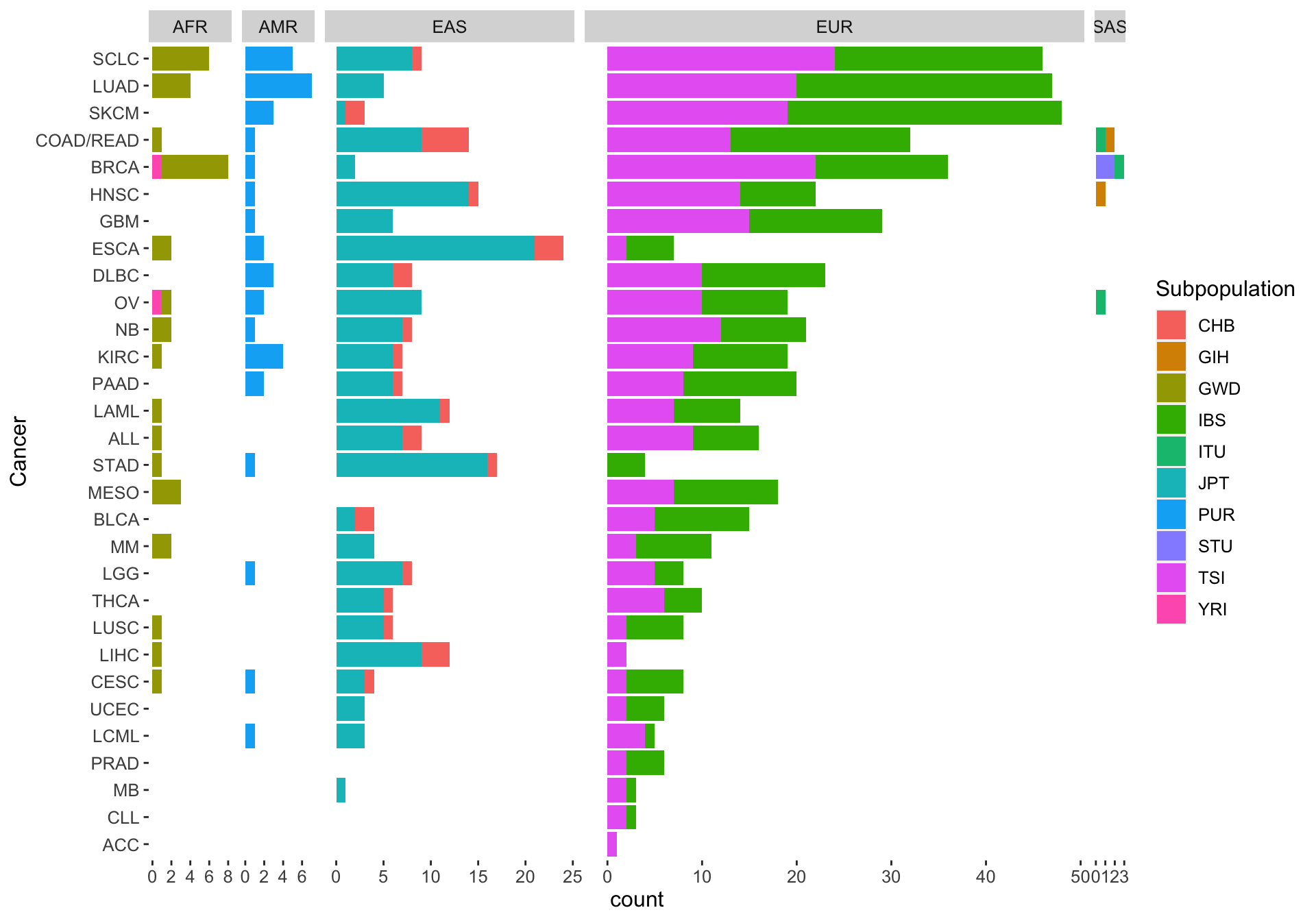
Ancestry distribution among cell lines and cancer types
Above is the step by step guide of how to infer ancestry from raw genotype data of cancer cell lines. The comprehensive pipeline could be found in my github repository for this project.